The World seen in Deforestation

This is a map of the world in ‘deforestation intensity’. Please click on it to see it full size.

Map of deforestation globally from 2000-2012, taken from Hansen et al. (2013).

I have replotted this from the original 30 m data to a 3 km resolution, and coloured each pixel according to the proportion it has been deforested over the time period:

Please do click the image to make it fill a browser window – you cannot really appreciate it in the narrow confines of a WordPress Blog!

I find it terrifying that every major landmass (save Greenland and Antarctica) is visible in this map. I haven’t added any borders or anything else: this is purely pixels coloured according to their deforestation. With the exception of central Amazonia, and the north-western United States, every major forested area in the world is lit up in this map.

What is particularly clear in this is the global hotspots of deforestation. Malaysia, Indonesia and the ‘arc of deforestation’ in Brazil are brightly lit up, as is to a lesser extent Siberia and some parts of the USA and Canada. The temperate and boreal forests showing big changes here are probably less of a global worry: though some of this loss is due to wild fires, storms, pests and disease, much of it is natural clearing in managed plantations and the losses will be replaced. There is in fact probably a net gain in forest cover in much of the world outside the tropics. The losses in the tropics however are very concerning, as most of this forest is being replaced by agriculture or severely degraded ecosystems.

We have run an analysis of the area of forest lost in each country globally. We found that an incredible 13.4 % of Malaysia has been deforested between 2000 and 2012, 7.9 % of Indonesia, and 4.0 % of Brazil. These figures are not a proportion of forest loss, but a proportion of the whole country that has been reported as undergoing forest loss over that period.

In some countries, notably Brazil, deforestation rates have reduced recently, with Hansen et al. (2013) finding a negative trend in deforestation rates. But in others, particularly in SE Asia and Africa, rates of forest loss are actively increasing.

If you want to explore this dataset more, please visit the excellent site set up by Matt Hansen in partnership with the Google Earth Engine team at this link, where you can view the data at its full 30 m resolution. Alternatively you can also view this and other data at the Global Forest Watch site.

Detecting deforestation by sound!

I’ve just found out about an amazing Kickstarter project, to raise money to use discarded mobile phones and solar panels placed on trees to act as detectors for deforestation. The sensors can pick up the noise of chainsaws from a mile away, and immediately transmit the signal using a mobile network.

The sensors look like this:

And here’s a schematic of how it works:

The organisation behind this is called Rainforest Connection, based, perhaps unsurprisingly given the innovative use of technology, in San Francisco. They have so far raised $125K of their $165K target, and have just 5 days left to go.

Details available at their website here Kickstarter page here.

I’m really looking forward to seeing how this gets on: it seems to me it would be great to combine real time information from a system like this in high risk areas, with satellite and community-led systems providing more regional coverage. Plus great to see a use for old phones that doesn’t involve landfill.

Free forest mapping graphics

For those of you interested in using LiDAR for forest carbon mapping, Iain Woodhouse has just posted some free forest mapping graphics produced by his spin-out company Carbomap. They look really nice – useful for lectures and your own web projects? Anyway, follow the link and see what you think.

Produced by Carbomap, shared under a creative commons licence

Link

Excellent post from my work experience student

I’m currently lucky enough to have a work experience student with me for 6 weeks this summer. He’s written an excellent blog post about his project – check it out!

First imagery from Landsat 8.

Good news for the detection of deforestation, but what are the implications of changes in sensor characteristics compared to previous satellites?

The series of Landsat satellites has provided a unique archive detailing changes in the land surface since 1972. The 8th satellite was launched successfully on February 11th 2013, and with on board checks and calibration complete, NASA handed it over to the United States Geological Survey (USGS) in May. Its first images have now been processed and are available to download free of charge via GLOVIS. I’m very excited because I’ve just downloaded and processed my first scene, over Sierra Leone and Liberia, including one of my study sites, the Gola Rainforest National Park:

Landsat 8 scene covering southern Sierra Leone and western Liberia, captured 2nd June 2013. This is a 6-5-4 composite, stretched to accentuate the difference between intact forest (dark green), degraded forest (light green) and non-forest (purple). Image courtesy of the U.S. Geological Survey.

Though there has been at least one Landsat satellite in orbit since Landsat 1 was launched in July 1972, there have been a few hiatuses (hiati?) in Landsat coverage, periods of time where few high quality images are available in the archive for much of the world. The most notable are in the early- to mid- 1990’s, caused by funding uncertainty, mis-management and the loss of Landsat 6 at launch; and November 2011 until May 2013.

This most recent gap has only been partial, with two satellites collecting some data: Landsat 7 was launched in 1999 but since May 31st 2003 it has had a fault with its Scan Line Corrector (SLC), causing the loss of some data within each scene. Landsat 7’s sensor (ETM+) is, like the TM sensor of Landsats 4 & 5, a whisk-broom sensor, which collects data via a mirror that scans side-to-side, parallel to the satellite’s track. The SLC is a set of two mirrors that corrects for the forward motion of the satellite to keep the scan lines parallel to each other. SLC-off data therefore has wedges of data missing:

The result of this is that 22 % of the image data is missing, in wedges that increase in size towards the edge of the image. Only the very center of the scene is unaffected:

Though Landsat 7 has continued to successfully collect data from this date onwards, the missing strips make using this data for land-use change difficult. Incredibly however another source of Landsat data is available, despite no new Landsat satellite being launched for almost 10 years after this date. This is because Landsat 5, a satellite launched on the 1st of March, 1984, continued collecting useful data until November 16th 2011, when a fault developed in its transmission system. While this has been partially fixed, and Landsat 5 recently set a Guiness World Record for the longest continuously operated satellite, at 28 years 10 months, it has been collecting little data since that point.

The commissioning of Landsat 8 is therefore very welcome. It will be widely used by a huge range of organisations, but my interest is particularly regarding its use for mapping forest cover changes to quantify deforestation and degradation. I intend to use Landsat imagery (clouds permitting) to update land-use change analyses I’ve already performed for sites in Sierra Leone, Cameroon, Gabon, Uganda, Peru and Colombia, and have begun downloading the necessary images, as you can see above.

Different sensor characteristics: OLI vs ETM+/TM

Before analysing these images though it is important to understand that the sensor on Landsat 8 differs in many ways from that found on earlier Landast satellites. That sensor characteristics should change with time as technology improves is only natural, and has happened before in the Landsat series. The primary Multi-Spectral Scanner (MSS) sensor of earlier Landsats was superseded by the Thematic Mapper (TM) sensor on Landsat 4 & 5, increasing the resolution to 30 m and increasing the number of spectral bands (though both also carried MSS sensors for data continuity reasons). Landsat 7 features a sensor called the Enhanced Thematic Mapper+ (ETM+), which was a relatively small update of the TM sensor – it  added a panchromatic band at twice the resolution (15 m) to allow finer details to be distinguished, however the spectral bands and basic design remained the same.

The Operational Land Imager (OLI) on Landsat 8 is very different to ETM+ however, representing much more than just an evolution of the earlier sensor. Its whole design is different: it is a pushbroom rather than a whiskbroom sensor, resulting in fewer moving parts (no SLC to go wrong here!) and a higher signal-to-noise ratio. But more importantly from a user perspective is that the wavelengths have changed: 3 new bands have been added, and most of the other bands now detect a smaller range of wavelengths:

Spectral bands of Landsat 8 vs Landsat 7 sensors. Note the additional bands in Landsat 8, and that the duplicated bands are mostly narrower. Image provided by NASA, source http://landsat.usgs.gov/ldcm_vs_previous.php

In theory these narrower wavelengths should improve the ability of the sensor to discriminate different landcover types, so they are good news. But the lack of continuity is a problem: a classification algorithm applied to one sensor should not be blindly applied to another anyway, but even with good cross-calibration doing so would not be appropriate here. Even the widely used NDVI will differ between the old and new sensors, with the near infrared band on OLI being much narrower than the equivalent band on previous satellites (compare OLI band 5 with ETM+ band 4 on the graph above). I will be performing some comparisons between near-contemporaneous Landsat-7 and Landsat-8 scenes over the next few months to see how much effect this has.

While changing wavelengths is in some ways unhelpful, the additional bands are another story. I’m particularly excited about the new Band 1, which is designed to help detect hazy, high-altitude cirrus clouds, which can be hard to spot but can subtly change spectral characteristics.

The future

Optical satellite data will remain a very useful tool far into the future, so I’m hopeful the Landsat dataset will continue to be added to for many decades yet. However, the US Congress has not as yet committed funding for any more Landsat satellites, and there is no long-term commitment by the US to keep Landsat series operating indefinitely. With the Landsat archive having been made open and free in 2008, and with scenes collected worldwide, Landsat provides an incredibly service to the rest of the world, but there is no guarantee this will continue.

With the need for continuous, consistent satellite data in mind, the EU is funding ESA to launch a series of Landsat-like satellites as part of its Sentinel series, part of the Global Monitoring for Environment and Security (GMES, now known as Copernicus) initiative. Sentinel 2 is based around a wide-swath, 10 m resolution sensor, with a pair of satellites able to provide images of the whole land-surface every 5 days. The first satellite will be launched in 2014, with partner and replacement satellites budgeted into the 2030’s, using technology and expertise developed from the SPOT satellite series among others. While there have been many other Landsat-like satellites launched in the past, and many are operational now, Sentinel 2 is the first that, like Landsat, will offer ‘free and open access for all’. I hope there will be a Landsat 9, but if not then it is good to know that Landsat 8 is there to bridge the gap between now and the start of the Sentinel era.

A step by step guide to making maps of vegetation carbon stocks

A follow on from the 5th Building Carbon Bridges across Africa workshop 

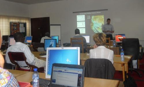
I’ve just come back from leading a training workshop in Accra, Ghana, as part of the Building Carbon Bridges across Africa project. For me this was a very useful and informative workshop, and I hope very much that the 12 participants from African government ministries and forestry departments learned some useful new skills. I’m writing this blog post to share some of the training I conducted in that workshop more widely. 

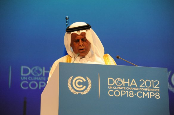
I want to start by explaining a bit about the Building Carbon Bridges initiative. Building Carbon Bridges is one of an increasing number of South-South collaborations for REDD+, funded by western organisations. Ghana has recently developed a high-resolution carbon map, and has considerable expertise on other aspects of the Monitoring, Reporting and Validation (MRV) process, creating registries, and integrating sub-national projects (“nesting”). This project was set up to allow Ghana to share its knowledge with some East African countries (Ethiopia, Kenya, Uganda & Tanzania) and Nigeria. Building Carbon Bridges was funded by the Clinton Climate Initiative and run by Ghana’s Nature Conservation Research Centre (NCRC) in partnership with the Common Market for East and Southern Africa (COMESA).

This workshop, the 5th and final in the series, was run by NCRC and Ghana’s Forestry Commission and held in the excellent remote sensing training facility in the Center for Remote Sensing and Geographic Information Systems in the University of Ghana. I did the majority of the teaching at the workshop, but sessions were also led by Rebecca Asare and Winston Asante of NCRC.

Below I summarise some of what we discussed over the 3-day workshop – in particular I will go over links to some existing datasets, discuss how they can be used, and introduce the concepts of how you can develop your own carbon maps.

Why carbon maps?

So, why would you need a map of vegetation carbon? I can think of several reasons, that apply whether you are responsible for a small forest reserve, a forest concession, a community forest, a province or the forest/environmental resources of a whole country:

1. Mapping carbon over your area of interest gives you an estimate of the total carbon locked up in the vegetation. This carbon has considerably value to the world: if it is released to the atmosphere it will contribute to climate change. Only by measuring this asset can it be valued. Forests have much more to offer the world than just their carbon stores (ecosystem services including flood protection, rain generation, evaporative cooling, and their store of biodiversity), but their carbon can be easily measured and doing so provides a part of the case for their preservation.
2. Carbon maps show the areas of high and low biomass within a region. This allows efforts at forest protection to be targeted to the higher carbon areas, or potential can provide a warning sign of areas subject to degradation.
3. Repeat carbon maps (for example annually, or every five years) allow calculations of net changes in carbon stocks. These net change numbers directly relate to payments under REDD+ or carbon sequestration schemes, and also can be used to set up historical baselines for carbon stock changes.

Why remote sensing?

The only way to accurately estimate the aboveground biomass of a forest is to set up field inventory plots, measuring the diameter and identifying the species of every stem (usually above a minimum size of 10 cm, as small trees do not contribute much to biomass), and measure the height of a subset. Standard methodologies exist for this, for example as described in the RAINFOR Plot Establishment and Remeasurement Manual.

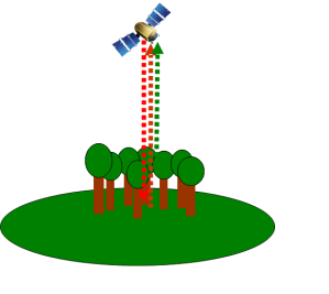However, most field plots only cover 1 hectare (or often less), and are very time intensive and expensive to set up. Remote sensing allows the whole landscape to be sampled equally, regularly, and with little or no cost to the user. Only remote sensing can provide the continuous and regular view of a landscape essential for carbon stock monitoring. But remote sensing instruments do not directly measure biomass – they only provide indirect estimates. So field data remains essential – the guidance for forest carbon projects is clearly that remote sensing and field data should be combined (for example as stated in the excellent GOFC-GOLD sourcebook, the authority on estimating and reporting carbon stocks.).

Definitions and units

Before we start, we should clear up some definitions:

• Aboveground Biomass (AGB): this is the oven-dry mass of all aboveground living plant material in a plot. Often in the literature only stems > 10 cm diameter (DBH) are included in calculations of AGB – this is fine in most forest ecosystems as most biomass is held in the large trees, but before reporting results a correction factor must be made to account for seedlings, shrubs and small trees. Units are normally in tonnes per hectare (Mg ha^-1)
• Carbon stocks: carbon makes up approximately 50 % of plant biomass, and so biomass can be converted to carbon by multiplying by 0.5. Stocks over a landscape are normally expressed in units of carbon, not biomass, as this makes more sense when collating other carbon pools not covered here (e.g. soil carbon). Normal units are MgC, TgC or PgC, depending on the size of area being measured. 
• tCO₂e: this is the number of tonnes of carbon dioxide that would have the same global warming potential as the material being discussed. In our case this is easy to calculate: we simply multiply the number of tonnes (Mg) of carbon by 3.667. tCO₂e are useful when comparing different types of carbon project, as the prevention of emission of other greenhouse gases (e.g. methane) can be converted to their CO₂ equivalent.

Image from UN Photo/Paulo Filgueiras.

What existing biomass maps are available?

There are two relatively high resolution maps of carbon stocks covering the tropics that can be freely downloaded by projects and used. A brief summary of how they are derived is summarised in a website I wrote here.

The first was developed by Sassan Saatchi and his collaborators, and was published in 2011 in the journal Proceedings of the National Academy of Sciences. A link to the original article can be found here. I should declare an interest at this point – I assisted in developing this map during my PhD, and am an author on the paper.

The second was developed by Alessandro Baccini and was published in the journal Nature Climate Change in 2012. A link to the original article can be found here.

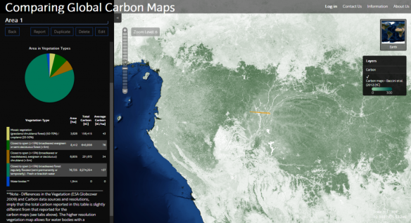
I have developed a simple web tool that allows you to visualise, compare and query the maps. I have blogged about this tool before. Alternatively, the authors have made the raw data for both their maps available online to any user. The Saatchi et al. map is available here, the Baccini et al. map here.

Some country-level maps also exist, for example Ghana has produced its own 100 m resolution map, but these are unfortunately rarely freely available online.

Simple map comparisons

These different carbon maps can be directly compared using the web tool described above.

However, to do more detailed comparisons and create maps, you will need to use a remote sensing or GIS software package. There are a number of open source GIS systems that are powerful and easy to use, including (in no particular order) GRASS, SAGA, and QGIS. There are also commercial packages: ArcGIS is the most widely used GIS software package, and due to its ubiquity this was used for the workshop. Most suited to developing carbon maps are true remote sensing packages, that can easily open, manipulate and analyse satellite datasets. I use IDL-ENVI for my research, and another packages with similar capabilities are ERDAS IMAGINE and IDRISI.

Any of the above packages should enable you to open the carbon maps described above and:

• Create output maps over an area of interest using the same stretch.
  
• Extract the mean and total biomass over your area of interest, or a subset
• Create maps of the differences between maps (using the Raster Calculator or similar function to subtract one map from the other)
• Use a landcover map (see below) to discover the mean biomass of different landcover types, and from that use a spreadsheet to estimate the likely carbon losses (or possibly gains) that would result from landcover change. For example, if your ‘broadleaved forest’ class cover 1000 ha and had an aboveground biomass of 300 Mg ha^-1, and ‘farmland’ had an AGB of 0 Mg ha^-1, if you lost 10 % of forest (i.e. 100 ha) you could calculate that you would lose 300 x 100 = 30,000 tonnes of biomass, or 15,000 tonnes of carbon, or and 54,900 tCO₂e (confused about the units? See the definitions sections above).

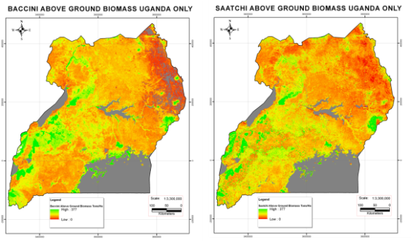
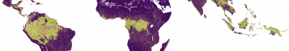
Comparison of two carbon maps over Uganda from BCB5 training workshop. Note the similarities (the location of high biomass areas are similar) and differences (e.g. more high biomass forest in the SW in Baccini et al. map).

Creation of maps from landcover classifications

If you would like to build your own carbon maps, rather than rely on published datasets, one of the simplest way is to use a landcover classification, and assign carbon values to different landcover classes. You may already have a landcover map for your region/country, or you can download an existing one. Two that are widely used are:

1. the Global Landcover 2000 (GLC2000) dataset, which was a 1 km resolution dataset developed for the year 2000. The data can be downloaded here.
2. the European Space Agency (ESA) GlobCover product, which is 300 m resolution and is available for the years 2005 and 2009. The datasets can be downloaded here.

In order to create a biomass map from a landcover map you need estimates of the biomass of each class. These are best obtained by locating a large number of field plots within each class; if that is not possible then a first guess can be made by matching the landcover types to values in standard tables, for example in forest inventory or FAO Forest Resource Assessment (FRA) reports for your country, the values in Annexe 3 of the IPCC’s Good Practice Guidance on Land Use, Land Use Change and Forestry.

Then a biomass map can be created using your GIS package, by assigning an AGB value to each class using a Reclass Table (or similar depending on your software).

Here is an example map produced at the workshop:

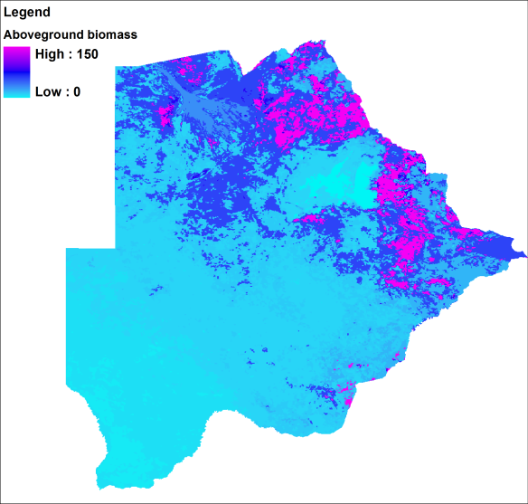
Botswana biomass map from GLC2000 landcover map and IPCC values

As you can see maps produced using this method are blocky, having a ‘painting by numbers’ look. This is because rather than each pixel being given a unique value, each class has the same value. Such maps have their uses, but clearly do not represent reality as do maps with different values for each pixel, which better reproduce the heterogeneity of ecosystems.

Creation of maps from active remote sensing data

By and large, optical datasets (e.g. Landsat, MODIS, SPOT) cannot be used for directly mapping biomass. They can be used for mapping landcover and landcover change, which is useful, but often have little sensitivity to biomass. This is a shame, as the vast majority of remote sensing data is optical.

However, fortunately, there also exists active remote sensing datasets, LiDAR and radar, which can map biomass at a pixel level (not having to go via landcover). Radar and LiDAR sensors have the capacity to produce accurate maps of biomass and biomass change, as shown in for example this paper of mine from Cameroon (radar), this from Gabon (lidar and radar fusion), or this paper by Greg Asner over Amazonian Peru (lidar and optical fusion).

In the workshop, we downloaded radar data over Africa from the ALOS PALSAR satellite, which is available freely form the Kyoto and Carbon Initiative website at a 50 m resolution for 2008 and 2009. This data is also available for SE Asia for 2008, 2009 and 2010; however unfortunately no free South America data is available currently. We then applied an equation from one of my papers (this one) relating radar backscatter to biomass, and from this were able to make biomass maps of the lower biomass regions and countries.

Backscatter:biomass equation from Mitchard et al. (2009):
EXP [(-2.73 + sqrt(7.45-(0.623(22+”Sigma0″))))/-0.311]

Unfortunately the ALOS PALSAR sensor is only sensitive to biomass up to about 150 Mg ha-1, so we were unable to map biomass over high biomass regions using this sensor. We were however able to use point estimates from the ICESat GLAS LiDAR sensor to estimate forest height, and hence biomass, in high biomass areas. ICESat GLAS data is freely available to download, but data was only collected from 2003-2009.

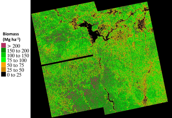
Biomass map over Mbam Djerem National Park in Cameroon. Derived from ALOS PALSAR data from 2007 and local field plot calibration. Details here.

Creation of maps from nonlinear models

When mapping biomass over very large areas, wall-to-wall coverage using active remote sensing data is not currently possible. Therefore combinations of field data, LiDAR/radar data, and optical data are normally used, combined using complex nonlinear models. This is the method followed by the two pantropical biomass maps described above.

There is not space here to describe the precisely methodologies used in detail – this is a complex process involving specialist software. See the Baccini et al. and Saatchi et al. papers for descriptions of how they did it – maybe I will expand further giving a step-by-step guide in a further blog post if there is interest.

Wrap up

I presented a summary of first steps for using aboveground biomass maps that already exist, and then mapping aboveground biomass in your study site. Obviously this is a very big topic, but I hope the above has provided help on the first steps, and links to useful resources. Please get in touch if this has been useful. Or if you have any questions or comments, please send me an email, or better still comment below so everyone can benefit.

Comparing Global Carbon Maps

I’ve been interested for a while now in comparing the many different regional and global maps of terrestrial forest carbon. Many of these maps have been produced recently, covering wide areas and making bold claims about their accuracy. They promise carbon forestry projects and countries a first estimate of their vegetation carbon stocks, which along with predicted deforestation rates allows them to estimate their potential income from a REDD+ project (though see this post for an update on the stalled international REDD+ process).

In partnership with Ecometrica I have produced an interactive website to compare these carbon maps. You can access the site here, read an article I’ve written about the new site for Ecometrica here, and access a website describing the site here.

As you can see, though in many areas the two maps agree, in some areas there are large disagreements. Ecometrica’s innovative Our Ecosystem platform, on which the site was built, allows you to draw a region of interest, compare the carbon stocks estimated by the two maps for different landcover types, and download these data as a pdf report. This should help projects understand better not just the carbon stocks in their forests but the uncertainties in current maps.

The two maps compared at the moment are by Saatchi et al., published in PNAS in 2011 (on which I am a co-author), and Baccini et al., published in Nature Climate Change in 2012. We are hoping to greatly increase the number of maps shown on this site in the near future: if you’d like to display your map on this interface please get in touch.

What next for forest conservation after disappointing Doha?

President of the Conference of the Parties (COP 18), Abdullah bin Hamad Al-Attiyah address the UN Climate Change Conference in Doha, Qatar. Photo: UNFCCC

Now the dust has settled the consensus appears to be that COP 18, held in Doha, was  yet another disappointment in the stalled UNFCCC process. Yes, the Kyoto Protocol was extended to 2020: but with only Europe and Australia are now parties to it, between them responsible for just 12 % of global greenhouse gas emissions, this is hardly grounds for optimism. Countries made next to no progress in closing the ‘Emissions Gap’ identified in a recent UNEP report, with current policies likely to take the world far beyond the 2 degree agreed maximum warming target of the UNFCCC. Furthermore next to no progress was made in talks on REDD+ (Reducing Emissions from Deforestation and forest Degradation): no agreement was made on the two most important areas – how it would be financed, and how it would be monitored.

This is disappointing. The ‘Durban Platform’, agreed at the COP17 conference in Durban in 2011, envisaged an all-encompassing agreement to limit global emissions, including for the first time developing as well as developed economies. It was to be signed by 2015, and to take effect in 2020. However, agreement on an effective comprehensive deal is now looking less and less likely, with developed and developing nations seemingly further apart after Doha than before. In 2012 atmospheric carbon dioxide concentrations reached a peak of 396 ppm (41 % higher than pre-industrial concentrations), while summer Arctic sea ice reached its smallest recorded extent ever,  the US had a record-breaking wildfire season triggered by record-breaking droughts, Hurricane Sandy wrecked havoc in the Caribbean and US East Coasts, and floods caused tragedies in places as diverse as the Philippines, North Korea, the UK, India, Peru and Nigeria. While floods and hurricanes cannot be directly attributed to the rise in carbon dioxide concentration, it is clear that recent global warming, strongest at the poles, led directly led to the reduction in Arctic sea ice. Hurricane Sandy was in all likelihood made more powerful due to exceptionally high sea surface temperatures and more devastating due to rising sea levels, and floods have always been predicted to become more common in a high CO2 world. Yet politicians failed to act, instead concentrating more on apportioning blame for past emissions. Indeed, as the case for action on climate change becomes stronger, political will to do something appears to be becoming weaker.

The inexorable rise in atmospheric carbon dioxide concentration continued in 2012.

But what does all this mean for the protection of tropical forests? REDD+ was meant to become a key part of a comprehensive climate change deal, and receive its funding from that process. If the Durban platform leads to nothing, does REDD+ die too, and with it the last hope for the world’s tropical forests?

I sincerely hope not. There seems to be a consensus forming that perhaps forest preservation is best done outside the main UN system. This is already happening at two different scales: at a local scale there are approximately 200 voluntary-sector REDD+ projects either currently functioning or in an advanced state of development; and at a national scale a number of programs exist to support whole countries in monitoring and managing their forests (e.g. UN-REDD and the FPCC), and a number of bilateral agreements exist, most famously the $1 billion Norway-Indonesia REDD+ Partnership. As small-scale projects grow and merge, and bilateral and regional deals become more numerous, it is possible that an international system to fund the protection of tropical forests could come to exist even without any overarching international framework. It will undoubtedly be more complicated, messier, and harder to monitor than a UNFCCC deal would have been, but that does not necessarily mean it will be less effective.

I’ll end this blog post on that positive note. However, a decentralised REDD+ scheme is not without pitfalls, and I’ll write about these (and potential solutions) at a later date.

Are Cameroon’s forests doomed?

A new map shows mining permits overlap many protected areas in Cameroon

The Interactive Forestry Atlas of Cameroon Version 3.0 has just been released by the World Resources Institute (WRI), giving spatial details on all the management units of Cameroon’s forests for 2011. The data have been released in the form of a report, an excellent interactive map, and the raw GIS files¹. While the report does not give data on rates of deforestation per se, it does show the location and status of forest and mining concessions, as well as the various categories of protected and non protected other forests.

I downloaded the data yesterday, and expected to spend this morning overlaying the active logging concessions on satellite imagery, to test my ability to detect forest degradation. However, opening the full dataset, I was immediately horrified by a different spatial layer. It appears that mining permits have now been issued for almost 10 million hectares of Cameroon, about a fifth of the country’s total area. 85 % of these overlap with forested areas, and 40 % of these concessions overlap forest designated by the government as ‘Permanent Forest Estate’, that is land that is meant to remain forest in perpetuity. Incredibly, 20 % overlap some form of protected area, and nine concessions overlap with National Parks.

Figure produced by Ed Mitchard using data from Data from the WRI Interactive Forest Atlas of Cameroon 3.0.

Mining permits are not all the same: most of these are exploratory, and do not allow for widespread extraction. However, for the government to issue them at all there must be an assumption in the Ministry of Mines that these exploratory permits could be converted to extractive permits if the companies involved find significant deposits. This surely should not be allowed within the official Permanent Forest Estate, let alone in national parks. It seems likely that officials high up in Cameroon’s government have given authority for the supposedly concrete forest protection areas to be changed if there are economically important mineral deposits underneath.

For me, the most breathtaking overlap is the two permits that cover 20 % of the Dja Biosphere Reserve in southern Cameroon. The Dja Reserve  is a UNESCO World Heritage Site and is one of the most important national parks in central Africa. It contains over 600,000 hectares of near-undisturbed rainforest, an area twice the size of Yosemite National Park, and has a unique assemblage of species. UNESCO has recently published a damming report stating that the Dja Reserve is critically threatened by a combination of mining, commercial agriculture, flooding from a planned hydropower dam, bushmeat hunting and illegal logging. I am part of an effort to set up a Reducing Emissions from Deforestation and Forest Degradation (REDD+) project in the area, funded by voluntary sector carbon credits, but such a project has little chance of success if Cameroon does not obey its own laws.

It is difficult to know what to suggest as a solution. I believe that Cameroon has the perfect right to develop, and to develop fast. It is a very poor country with significant unexploited mineral and forest resources, and the reasoning behind this push into mining and commercial agriculture is to build up its economy. This rush towards industrial development is a key pillar in Cameroon’s Vision 2035, a 2009 document which tracks a path to Cameroon becoming a major emerging economy by 2035. However there is a concern, which I share, that the costs of this industrialisation will be borne mostly by the poor, who will be displaced from their land, have their drinking water polluted, and lose their livelihoods. Meanwhile, the benefits will be felt mostly by those who are already rich. Equally I am concerned by the rapid destruction of the country’s natural heritage, with no national or international debate. Open cast mines elsewhere have caused significant environmental damage, removing all vegetation, causing massive erosion, and permanently scaring the landscape.

Open Cast mine in the Philippines.
Picture (c) Storm Crypt, reproduced here under a Creative Commons license.

Cameroon shouldn’t need to grow at the expense of its natural environment. As a country I believe it has so much potential – it has plentiful natural resources, incredible wildlife and a wealth of cultures (over 230 languages are spoken). The wildlife and cultures remain largely intact, and it’s possible to extract the other natural resources without destroying them. Cameroon’s process for allocating forestry concessions is much more transparent than it once was, and Cameroon is now actively involved in reducing illegal logging through the EU’s FLEGT program. If that were to continue and expand, Cameroon could earn a significant income from the sustainable logging of its precious hardwoods while maintaining its protected area network, safeguarding biodiversity and earning further income through ecotourism. Agroforestry programs, involving for example the sustainable growth of cacao to feed the world’s ever-increasing demand for chocolate, could be expanded. Local people, including traditional forest dwellers, could be involved in decisions of whether to explore for minerals or oil, how to extract them, and could share the proceeds.

The external world can help by monitoring what is happening (hence the great utility of this WRI effort) and applying pressure, as well as providing sensible solutions that work for the poor as well as the rich (in terms of both people and countries , for example a well-designed international REDD+ agreement.

¹The GIS files that make this map can all be downloaded here, for 2004-2011. WRI and Cameroon’s Ministry of Forestry and Wildlife (MINFOF) should be congratulated for providing these: there is a huge difference between making a report visible online and releasing the underlying data. Having been involved in many conservation projects in African countries I know how difficult and frustrating it can be to obtain baseline spatial data – I have for example before had to spend days painstakingly hand-digitising pdf maps. I am sure the shapefiles will be widely used.

Measuring trees in Gabon

I’ve just spent 8 days in an isolated Shell oil camp in the rainforests of Gabon. The accommodation is luxurious shipping containers:

View coming into land in the Shell Gabon Rabi camp.

But the food is plentiful and there is a 25 hectare (that’s 500 m x 500 m) Permanent Sample Plot located in the forest just 1 km from the camp. This forest plot is part of the extraordinary global network of Center for Tropical Forest Science (CTFS) plots, funded by the Smithsonian Institute and local partners (including, in this case, Shell Gabon). There are now 47 plots globally, ranging from 25 – 150 hectares in size, where every tree from 1 cm in diameter upwards has been tagged, and their diameters measured.

This is a much smaller minimum diameter than is normally used (10cm is a more standard minimum for Permanent Sample Plots, which involves measuring typically just one tenth as many trees), and the plot sizes are much larger (just 1 hectare is more normal). The CTFS plot in Gabon has involved individually tagging and recording almost 200,000 trees.

The CTFS plots are an incredible resource for scientists trying to understand forest ecological processes (providing data to explain for example why tropical forests have so much higher biodiversity compared than other ecosystems). However, I’m here to use the data in a less conventional way.

I am working as part of an international consortium to assist the Gabonese government in mapping their forest resources, and in particular their forest carbon. As part of this effort I have previously produced a map of carbon for Lopé National Park using radar data, and used other field data to produce preliminary maps across Gabon. However, we realised that in order to do a good enough job to inform policy makers in Gabon and feed into the international REDD+ process we really needed a combination of a network of field plots across the country and aircraft-borne LiDAR data.

LiDAR data provides a highly detailed map of forest canopy height, by sending vertical pulses of laser light and detecting the time for the return signal: the difference between the first and last returns corresponds to the height of the canopy. This gives a very detailed map of canopy height, as well as information on canopy structure, but without good field data on tree heights from the ground we are unable to convert this height data into biomass.

Measuring the height of a tree with a Vertex Hypsometer

I have therefore been spending time at the CTFS Rabi plot measuring tree heights – our team of 6 people measured the height of just over 1200 trees in total, with the tallest tree 72 meters tall! I will use these tree height data for two purposes:

1) To create a ‘Gabon lowland rainforest’ specific equation relating tree diameter to tree height. Diameter is easy to measure in the field, whereas height is not, but they are closely related relatively consistently within most forest types – once we have a good equation, we can estimate tree biomass with much higher certainty from a simple diameter measurement.

2) To make a 3-D computer model of the Rabi plot, to compare to the aircraft-based LiDAR data that will hopefully be collected soon. I will compare the two to assess how accurately we can model this patch of forest from LiDAR data alone.

I strongly believe that collecting all this field data will lead to better maps of aboveground biomass, which is very important for a wide variety of forest carbon initiatives. But in addition to this, as a remote sensing scientist it’s very easy to do all your work from a computer and become separated from the reality of what you’re working on. I therefore love doing fieldwork to keep in touch with the complexities of the forest ecosystems I study, and also to make links with local collaborators. Too often remote sensing studies do not include scientists from the country studied – for me providing training and exchanging ideas with local researchers is an essential part of my work.